Welcome to my third post in a series of topics on MDX for SQL University. If you’re just now joining me, you should check out the first post, Location, Location, Location, and my previous post, Writing Simple Queries, to get oriented. I’m going to continue building on the concepts introduced in the earlier posts by showing you how to use functions to create a set to use on an axis.
Many times you’re interested in seeing values for all of the members of a particular attribute hierarchy. For example, in this query, we can see sales for all categories and for all years, including a grand total for categories and years and also years that have no sales.
SELECT
[Date].[Calendar Year].Members
 ON COLUMNS,
[Product].[Category].Members ON ROWS
FROM [Adventure Works]
WHERE [Measures].[Sales Amount]
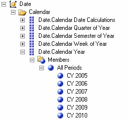
When you use the Members function with a dimension and hierarchy, you get everything listed in the Members folder:
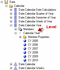
What if you don’t want the All Periods member to show up? Well, you could create a set like this {[Date].[Calendar].[CY 2005], [Date].[Calendar.[CY 2006], …} but that would be tedious, and it wouldn’t automatically include new members that get added to the dimension over time. Instead, you can use the Members function with the dimension, hierarchy, and level reference to skip over the All Periods like this:
SELECT
[Date].[Calendar Year].[Calendar Year].Members
 ON COLUMNS,
[Product].[Category].Members ON ROWS
FROM [Adventure Works]
WHERE [Measures].[Sales Amount]
Here we have a case of “more is less.” When we use a level reference, such as we do with the expression [Date].[Calendar Year].[Calendar Year].Members, we are providing more specific instructions to the Members function so that we can get less data. Using a level reference works with both attribute hierarchies (the ones with two levels only) and user-defined hierarchies (the ones with multiple levels and a pyramid-shaped icon).
One more little change to this query might make it better. If we don’t want to see CY 2009 and CY 2010 columns when they are empty, we add the NON EMPTY keyword in front of the set definition like this:
SELECT
NON EMPTY [Date].[Calendar Year].[Calendar Year].Members
 ON COLUMNS,
[Product].[Category].Members ON ROWS
FROM [Adventure Works]
WHERE [Measures].[Sales Amount]
What if we want to see the category sales broken down not only by year, but also by sales territory? We can combine sets on an axis using the CrossJoin function like this:
SELECT
NON EMPTY [Date].[Calendar Year].[Calendar Year].Members
 ON COLUMNS,
NON EMPTY
CrossJoin([Product].[Category].Members,
	[Sales Territory].[Sales Territory Group].[Sales Territory Group].Members)
ON ROWS
FROM [Adventure Works]
WHERE [Measures].[Sales Amount]
The CrossJoin function takes only two arguments, but you can use that expression as one argument in a second CrossJoin function to create a grouping of three dimension hierarchies on an axis. There are several ways to get the crossjoin effect which might be easier to read when you start adding more dimension hierarchies to the mix. One is the use of a “polymorphic operator” such as an asterisk * like this:
[Product].[Category].Members *
[Sales Territory].[Sales Territory Group].[Sales Territory Group].Members
The other is to create a tuple set like this:
([Product].[Category].Members,
[Sales Territory].[Sales Territory Group].[Sales Territory Group].Members)
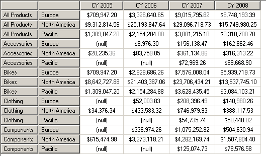
I know I said in a previous post that a tuple is like a coordinate to a cell, and it appears in the above example that I’m violating that rule by using sets in a tuple. But Analysis Services resolves this expression as a set of tuples by taking every member of the first set (the product category members) to create a tuple with every member of the second set (sales territory group members). That set gets placed on the rows axis and the set of calendar year members gets placed on the columns axis, and then the tuple coordinates for each intersection of a row and a column produces a new tuple definition that generates a result, such as $709,947.20 for the pseudo-tuple (All Products, Europe, CY 2005).
There are many more functions that we can use to generate sets to control what we see on rows or columns. More than I can cover in this post. (In fact, there are entire books that cover this topic. In a future post, I’ll provide some recommendations.) For now, I’ll leave you with one more function to add to your repertoire. This time we want to see only those product categories and sales territory combinations that have sales greater than $1 million in CY 2008, but we want to see their sales for all years. To do this, we use the Filter function. This should satiate your desire to use a WHERE clause in your query, which I told you in my previous post does not work like a filter as it does in a T-SQL query.
SELECT
NON EMPTY [Date].[Calendar Year].[Calendar Year].Members
 ON COLUMNS,
Filter(
	([Product].[Category].[Category].Members,
		[Sales Territory].[Sales Territory Group].[Sales Territory Group].Members),
	([Measures].[Sales Amount],[Date].[Calendar Year].&[2008])  > 1000000)
ON ROWS
FROM [Adventure Works]
WHERE [Measures].[Sales Amount]
The Filter function takes two arguments. The first is the set that you want to filter. And the second is a Boolean expression that determines which members will be in the set that the Filter function produces. In this case, I used a tuple expression to focus on the 2008 sales. If I had used only Sales Amount, the filter would have produced a set of category/territory combinations having total sales for all years greater than $1 million.
The key concept to take away from this post is that sets go on rows and columns, and that we can control very precisely which members are in those sets by using functions and tuple sets. A very common function to use is the Members function, and it’s also common to use NON EMPTY to rid ourselves of rows or columns that contain only null values.


4 Comments
[…] my recent series was of MDX posts, ending with A Gentle Introduction to Sets, was intended merely to be an introduction to MDX, and not a full-fledged course, I have a few more […]
Thank you for the posting, I am able to finally understand the concepts of tuple and members. I am looking forward for your book or future book in writing simple MDX queries.
Best wishes in your next endeavor!
sardys
Thanks, Sardys! I’m glad to help demystify MDX. No plans to write a book on simple MDX queries, but I will be adding more posts on the topic in the weeks and months to come!
Oh great to hear from you!! I love your postings. They are simple enough to understand MDX, and at the same time interesting enough to keep my curiosity engaged.