 This is the fifth and final post for SSAS week at SQL University. If you’re just joining the class, you should review the previous lessons first:
- Why Do I Need a Cube & How Do I Get Started
- Dimension Design 101
- Cube Construction 101
- Cube Enhancements 101
Today, I’ll show you how to secure access to the cube. I’ll also shed a little light on what happens when you deploy a cube, and I’ll wrap up this week’s lesson by explaining different ways that people might access a cube. There is so much more to learn about cubes when you have advanced analytical needs to support, but at the conclusion of this series you will have a grasp of the important concepts which is enough to get started with simple analytical requirements.
Security
Right now, you’re the only person who can browse the cube because you’re the one who created it. Before other people can browse the cube, you need to grant them the necessary permissions. Analysis Services supports only Windows integrated security, so everyone requiring access to the cube must have a Windows account. Rather than assign permissions to individual users, you might consider creating a Windows group and assigning users to that group.
Let’s assume that you have created a Windows group called SSAS and you’re now ready to set up security for your cube. Open your project in BIDS, right-click the Roles folder, and select New Role. The default name of the role is Role, but you can change that later if you like. Open the second tab in the role designer, Membership, and click the Add button. Locate the SSAS group to add the group to the role. Then go to the Cube tab and select Read in the Access drop-down list. In most cases, this step is the only one you need to perform. After you deploy the cube, anyone in the group can browse the cube using their tool of choice (which is not BIDS; BIDS is used by developers only).
Analysis Services also allows you to apply more granular permissions. For example, you can prevent users from viewing specific members in a dimension, such as the Mountain Bikes subcategory. You even prevent users from viewing certain cell values, such as the Sales Amount Quota for the AWC Logo Cap in 2008. As you might imagine, the subject of security is pretty deep and beyond the scope of what I can cover in an introductory course in SQL University. So instead, I’ll refer you to Granting User Access for an overview of security concepts in Analysis Services. For data-driven security, take a look at Analysis Services—Data Driven Security Model.
Deployment
Throughout this course, I have asked you to deploy your project to make it available for browsing. The Deploy command in BIDS actually performs three steps for you that can be performed individually by using alternative means:
- Build – In this step, BIDS combines all the files in your project (data source, DSV, cube, dimensions, etc.) and creates a single file that has the asdatabase extension. Essentially, it’s one giant XML file that contains all the definitions about database objects that you see as individual files in BIDS. It’s very common in production environments that developers cannot deploy objects themselves, but instead provide files and scripts for administrators to perform the deployment. If necessary, you can use the Build command in BIDS to generate the asdatabase file and deliver it to your administrator.
- Deploy – The administrator copies the asdatabase file to a location on the server hosting Analysis Services. Then, from the Microsoft SQL Server 2008 R2\Analysis Services program group, the administrator launches Deployment Wizard. (You can learn more about the wizard at Using the Analysis Services Deployment Wizard.) This wizard steps through the process of taking the asdatabase file from its current location, and moving it to the OLAP data folder of the Analysis Services instance where the file gets “unbundled” into separate database object files, just like the ones you had in BIDS.
- Process – The presence of the database object files is not enough to render the cube usable. Processing must take place first. Processing reads the definition files to determine how to get to the source data, how to query the data, and how to load the data into the structures that Analysis Services requires. After processing completes successfully, everyone (with permissions, of course!) can browse the cube.
Processing
You can connect to Analysis Services by using SQL Server Management Studio (SSMS), and then use Object Explorer to locate a database for processing. You can even access individual measure groups or dimensions for processing. There are different types of processing that you can do. When you’re still learning about Analysis Services, it’s generally best to do a full process of dimensions and then a full process of cubes. When you perform a full process of any dimension, each cube with which it’s associated will also require a full process and the cube will be unavailable to users during this time. As you learn more, you’ll find that you can perform other types of processing that keep the cube available, but require more thought about data preparation. An overview of processing options is available at Processing (Analysis Services – Multidimensional Data).
Usually, it’s not practical to process manually in SSMS every time that you want to refresh the cube. Most people create an Integration Services package that contains one or more Analysis Services Processing Tasks, and then schedule the package to run on a periodic basis.
User Access
Once a cube is deployed and processed, users with the appropriate permissions can connect to the cube and browse to their hearts’ content. Using what? Whatever Analysis Services client they have available. Most organizations that have Analysis Services in-house also have Microsoft Office. Users can create pivot tables to explore data in a cube. The user experience in Excel 2003 is not so great, but Excel 2007 or Excel 2010 work similarly.
Assuming you are using Excel 2007 or higher, you must create an Office Data Connection (ODC) file – or open an ODC file – first. To create the ODC file, click From Other Sources on the Data tab of the ribbon, and then select From Analysis Services. Provide the server name (or localhost) and click Next. Then select your database—My SSAS DB—and the cube—Sales—and click Next. You can use the Browse button to save the ODC file in a specific place, either a local drive for personal use or a SharePoint Data Connections library for shared use.
When you save an ODC file to SharePoint, it can be used for workbooks accessed using Excel Services, or for status indicators (aka KPIs) or Filter Web Parts in SharePoint. Working with ODC files for Analysis Services sources and configuring SharePoint to authenticate with Analysis Services correctly can be tricky. You can learn more at Plan Excel Services data sources and external connections (SharePoint Server 2010). If you’re using SharePoint 2007, refer to Plan external data connections for Excel Services instead.
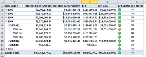
Regardless of where you save the ODC file, you use it as the source for a pivot table. In fact, after following the steps above and right after saving the file, you’re prompted for the location in which a pivot table will be inserted. On the right side, you should see the PivotTable Field list which displays all the measures by measure group, followed by KPIs and dimensions. All you need to do is select checkboxes for items that you want to display in the PivotTable, such as Internet Sales Amount, and Reseller Sales Amount. Expand the KPIs folder to add the following: Value, Goal, Status, and Trend. Also add Date.Calendar. Click the plus sign next to 2008 and 2008 Q1 to drill down to months. Your pivot table will look like this:
The KPIs aren’t very interesting with this data set because the total sales in the cube always exceeds the goal except when you drill down to months. The goal comes from the FactSalesQuota and is associated with quarters, but those quarters are referenced by the first day of the quarter, such as January 1, 2008, so the goal for January shown here is really a quarterly goal. There are tricks that we can use to either hide that value at the month level or to spread the quarterly amount across months in some way, but that’s beyond the scope of this week’s lessons. Hint for the curious: you have to add expressions to the MDX Script.
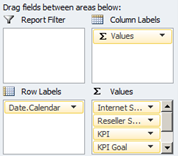
The selections you make in the PivotTable Field list appear below the list as objects that you can rearrange as desired. You can move dimensions from row labels to column labels or to the report filter. You can also drag the measures in the Values box to a higher or lower position to re-sequence the measures any way you like.
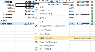
Remember in a previous lesson that you added an action to the cube. Let’s see how that works now. Right-click on one of the cells in the pivot table – such as the value $1,340,244.95 at the intersection of Jan 2008 and Internet Sales Amount, then point to Additional Actions, and then click on Internet Sales Details.
The action definition shows only the columns that you defined for the drillthrough action:
Excel also has a built-in drillthrough functionality that you can launch by just by double-click a cell value—as long as it’s not a calculated measure. The difference between the built-in functionality and the drillthrough action is that you have control over the columns that appear in the drillthrough action. It’s better when there is a specific set of columns that users want to see all the time, and is useful when you have a lot of columns available in a measure group and just want to focus on a subset of columns.
Your cube is also accessible for use with other tools. If you have a Reporting Services instance, users can launch Report Builder, select the Microsoft SQL Server Analysis Services provider type to create a data source, and then create a dataset using a designer interface that lets them use drag-and-drop to select the dimensions and measures they want to include in the report. User can also create status indicators from a cube for use in lists or SharePoint dashboards by using ODC files. If users want to access cube data in PerformancePoint Services scorecards and dashboards, a separate data connection for Analysis Services must be created.
Learning More
By completing the lessons in this introductory course to Analysis Services, you have the basic knowledge necessary to build simple cubes. But there is so much more to learn! Keep an eye on this blog as I’ll post topics related to Analysis Services from time to time, and of course SQL University will offer intermediate and advanced lessons in future semesters.
If your measure group contains fewer than 20 million rows, such as our sample cube from the lessons this past week, then you don’t need to worry about scaling the cube. Most business data these days contains many millions of rows, so enhancing the cube with scalability features is often the next step. The first step towards scaling is the addition of aggregations which you can learn more about by reading Optimising Aggregations in Analysis Services 2008. Another option to use, often hand in hand with aggregations, is the implementation of partitions.
A good online resource for all things related to Analysis Services is the Analysis Services Resource Hub. If you like to learn from books, here are several that I recommend:
- Microsoft SQL Server 2008 Analysis Services 2008 Step by Step by Scott Cameron, who started his BI career with me back in 1999.
- Professional Microsoft SQL Server Analysis Services 2008 with MDX by a line-up of Microsoft folks: Sivakumar Harinath, Robert Zare, Sethu Meenakshisundaram (who later went to SAP), Matt Carroll, and Denny Guang-Yeu Lee. Denny and I shared an office once upon a time before he joined Microsoft. It was entertaining, to say the least!
- Expert Cube Development with Microsoft SQL Server 2008 Analysis Services by SQL Server MVPs and friends Marco Russo, Alberto Ferrari, and Chris Webb.
- When you’re ready for advanced (really advanced!) material, tackle Microsoft SQL Server 2008 Analysis Services Unleashed by Microsoft developers who worked on the product, Irina Gorbach, Alexander Berger, and Edward Melomed. This book is required reading if you want to become an SSAS Maestro!


2 Comments
Thanks Stacia,
Great stuff as usual! As a “cube n00b”, posts like these really shed a lot of light on what is happening for me.
What strategy would you recommend to for handling null values? Not by my choice, the ETL doesn’t provide a default so we are left to deal with them in processing of the cube. Things look fine in the presentation layer (excel & web intelligence), but I’d like to be more proactive during process time in hopes we are ready for new ones. Would you recommend using isnull or coalesce in the TSQL view layer to prevent something like the following?
Errors in the OLAP storage engine: A duplicate attribute key has been found when processing: Table: ‘dbo_dim_D’, Column: ‘field1’, Value: ”. The attribute is ‘field1’.
When the distinct tsql runs to extract field1 data from the view, both empty string and null rows are listed, so SSAS introduces a dupe when it converts null to empty string by default… I believe
…or is there something I’m missing?
Thanks in advance!
~Tim
Hi Tim,
I would recommend using the DSV to clean up the nulls – you can use either the isnull or coalesce function as noted. But another option is to convert those nulls to the unknown member as per this article: http://technet.microsoft.com/en-us/library/ms170707.aspx.
Cheers,
Stacia